Contents
1. Model & Setup
All experiments use the LlamaGen GPT-B architecture with VQ-VAE tokenized ImageNet:
GPT-B Architecture
110M params, 24 transformer layers, 12 attention heads, dim=768. Causal attention with 2D RoPE spatial encoding. Block size = 256 (16×16 spatial grid). VQ vocab = 16,384.
Datasets
IN-100: ImageNet-100 subset, ~127K training images, 5K FID evaluation samples.
IN-1K: Full ImageNet-1K, 1.28M images, with pretrained c2i_B_256.pt checkpoint (300ep).
Shared Training Hyperparameters
All from-scratch models: batch=256, lr=1e-4, weight_decay=5e-2, max_grad_norm=1.0, dropout=0.1, token_dropout=0.1, bf16 mixed precision, 4×H100 GPUs, AdamW optimizer.
Evaluation Protocol
FID-5K and sFID against validation reference NPZ. Sampling: cfg_scale=2.0, temperature=1.0, top-k=0. All methods infer in raster order (standard left-to-right, top-to-bottom) unless noted otherwise. OrderHead uses semifast-8 (8 rescoring candidates).
2. Heuristic Orderings (Inference-Only)
Method
Take the raster-trained GPT-B baseline and evaluate it at inference with different spatial orderings.
The model weights are frozen — only the token generation order changes. Uses the sample_c2i_heuristic_ddp.py
O(L²) full-forward sampler that recomputes attention at each step with position_ids
for correct 2D RoPE per-token positioning.
Why O(L²)?
Standard KV-cache sampling assumes a fixed order (raster) so each new token simply appends to the cache. Non-raster orderings break this assumption: token at spatial position (5, 3) might be generated at step 10, requiring correct RoPE encoding for position (5, 3) but causal masking that only sees the 9 previously generated positions. The full-forward sampler recomputes from scratch at each step, giving O(L²) complexity (vs O(L) for KV-cache).
ImageNet-100 (5K samples, cfg=2.0)
| Ordering | FID | sFID | Source |
|---|---|---|---|
| Raster (baseline) | 25.40 | 66.33 | samples_fid_baseline_in100 |
| Raster (heuristic sampler) | 25.63 | 66.15 | samples_fid_heuristic_raster_in100 |
| Zigzag | 71.69 | 82.08 | samples_fid_heuristic_zigzag_in100 |
| Diagonal | 117.58 | 93.89 | samples_fid_heuristic_diagonal_in100 |
| Stride-2 | 128.18 | 93.83 | samples_fid_heuristic_stride2_in100 |
| Spiral | 132.25 | 97.06 | samples_fid_heuristic_spiral_in100 |
| Column-major | 139.79 | 100.69 | samples_fid_heuristic_col_major_in100 |
| Center-spiral | 153.53 | 111.03 | samples_fid_heuristic_center_spiral_in100 |
| Reverse | 156.18 | 109.45 | samples_fid_heuristic_reverse_in100 |
| Random (seed=0) | 173.08 | 119.23 | samples_fid_heuristic_random0_in100 |
Raster baseline from standard KV-cache sampler; all others from O(L²) heuristic sampler. The ~0.2 FID gap between the two raster results is sampling variance.
ImageNet-1K (5K samples, cfg=2.0, pretrained c2i_B_256.pt)
| Ordering | FID | sFID | Source |
|---|---|---|---|
| Raster | 5.32 | 7.46 | samples_fid_heuristic_raster_1k |
| Stride-2 | 119.62 | 45.38 | samples_fid_heuristic_stride2_1k |
| Center-spiral | 132.08 | 53.35 | samples_fid_heuristic_center_spiral_1k |
| Random (seed=0) | 151.23 | 66.11 | samples_fid_heuristic_random0_1k |
| Reverse | 154.35 | 68.76 | samples_fid_heuristic_reverse_1k |
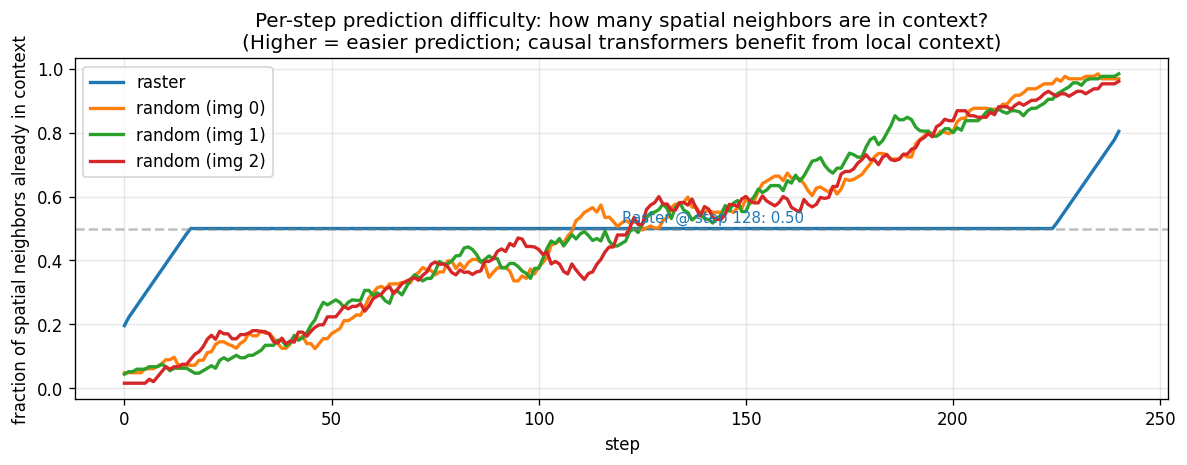
Spatial neighbor coverage comparison. At step 32, raster order has 34.8% of spatial neighbors already generated; random order has only 5-6%. This explains why raster is superior for causal AR: more context from immediate neighbors.
Takeaway: The raster-trained GPT is tightly coupled to raster context patterns. ANY deviation at inference degrades FID by 3x-7x. The 2D RoPE correctly encodes spatial position, but the causal attention pattern (which positions appear in left-context) is fundamentally different for each ordering.
3. Trained Orderings (From Scratch, IN-100)
Method
Train GPT-B from scratch on IN-100 with a fixed spatial ordering. Each model always sees tokens in the same deterministic order (e.g., always diagonal, always column-major). At inference, the same ordering is used with the O(L²) heuristic sampler.
- Training script
train_c2i.py(standard raster) ortrain_c2i_random_order.pywith fixed permutation- Epochs
- 300
- Batch / LR
- 256 / 1e-4
- Inference
- Same ordering as training, O(L²) heuristic sampler, cfg=2.0
| Training Order | FID | sFID | Source |
|---|---|---|---|
| Full raster retrain (fine-tuned from pretrained) | 17.57 | 67.18 | samples_fid_raster_ft_full_in100 |
| Diagonal | 24.97 | 65.99 | samples_fid_train_diagonal_in100 |
| Raster (original checkpoint) | 25.40 | 66.33 | samples_fid_baseline_in100 |
| Column-major | 25.95 | 66.26 | samples_fid_train_col_major_in100 |
| Zigzag | 26.35 | 66.18 | samples_fid_train_zigzag_in100 |
| Spiral | 30.94 | 66.42 | samples_fid_train_spiral_in100 |
| Random (one fixed permutation) | 44.74 | 66.78 | samples_fid_train_random_fixed_in100 |
Note: "Full raster retrain" is fine-tuned from the IN-1K pretrained checkpoint (300ep IN-1K + 300ep IN-100 = ~600ep effective), making it an unfair baseline. All others are trained from scratch for 300 epochs.
Partial Fine-Tuning (raster order, from pretrained c2i_B_256.pt)
| Layers Fine-Tuned | FID | sFID | Source |
|---|---|---|---|
| All layers | 17.57 | 67.18 | samples_fid_raster_ft_full_in100 |
| Last 4 blocks | 58.68 | 67.64 | samples_fid_raster_ft_partial4_in100 |
| Last 2 blocks | 92.69 | 70.41 | samples_fid_raster_ft_partial2_in100 |
| Last 1 block | 98.62 | 71.92 | samples_fid_raster_ft_partial1_in100 |
Takeaway: When trained with a specific ordering, most fixed orderings achieve FID comparable to raster (24.97–26.35). The ordering itself matters less than training/inference consistency. A random fixed permutation is worse (44.74) because the spatial context pattern is less structured. Diagonal is best (24.97), slightly beating raster (25.40).
4. Random-Order Training (v1, No Fixes)
Method
First attempt at random-order training in LlamaGen: every training step samples a new random permutation per image. Unlike a fixed ordering (Section 3), the model sees a different token order every step. This is inspired by MAR's random masking, but applied to causal AR.
- Training script
train_c2i_random_order.py(before RAR fixes)- Key difference
- No target-aware positional embedding, no annealing schedule
- Epochs
- 300 on IN-100
- Inference
- Both raster and random tested
| Inference Order | FID | sFID | Source |
|---|---|---|---|
| Raster | 159.41 | 115.89 | job 6474613 |
| Random (seed=0) | 163.98 | 121.23 | job 6474613 |
Root cause analysis: Two critical missing components identified by comparing with the RAR paper (arXiv 2411.00776): (1) No target-aware positional embedding — the model cannot distinguish permutations that share a prefix but differ in the next token (the "ambiguous target problem"). (2) No annealing to raster — raster inference is out-of-distribution for a purely random-trained model. Training loss plateaued at 8.45 (vs 6.30 for raster baseline). Generated images show realistic textures but no object structure.
5. RAR: Random Ordering with Annealing to Raster
Overview
RAR (Random-order with Annealing to Raster), based on arXiv 2411.00776, is a training curriculum that first trains with random token orderings and then gradually anneals back to raster order. The final model generates in standard raster order at zero additional inference cost — no architecture change, no extra sampling complexity.
Training Details
- Training script
train_c2i_random_order.py- Base model
- GPT-B (110M), trained from scratch (no pretrained init)
- Optimizer
- AdamW, lr=1e-4, weight_decay=5e-2, fused=True
- Batch size
- 256 global (64 per GPU × 4 GPUs)
- Grad clipping
- max_grad_norm=1.0
- Precision
- bf16 mixed precision
- Regularization
- dropout=0.1, token_dropout=0.1
- Hardware
- 4× H100 (1 node)
- Steps/epoch
- ~494 (127K samples / batch 256)
Two Critical Components
1. Target-Aware Positional Embedding (ta_pos_table)
A learnable nn.Embedding(256, 768) table. At training step t with permutation
perm, the token being predicted at position perm[t] receives the embedding
of perm[t+1] — the next token's spatial position.
Why it's needed: Without it, two different permutations that share a prefix but differ in the next token produce identical inputs to the model. The model cannot distinguish “predict position (3,5) next” from “predict position (7,2) next” given the same context — the ambiguous target problem. This makes optimization ill-posed.
Implementation: Zero-initialized (starts as a no-op). Added to GPT's token embeddings
during the random and annealing phases. Set to None during the pure raster phase and at
inference, since raster order is unambiguous (next position is always spatially adjacent).
Included in AdamW optimizer with the same LR and weight decay as GPT.
2. Annealing Schedule
A random_ratio controls the probability that each sample in a batch uses a random
permutation vs. raster order. The schedule has three phases:
- Random phase (epochs 0–150):
random_ratio=1.0. Every step draws a fresh random permutation per image. Model learns to handle arbitrary context subsets. - Annealing phase (epochs 150–225):
random_ratiolinearly decays from 1.0 to 0.0. Each sample independently draws random vs. raster. ta_embed active when random. - Raster phase (epochs 225–300):
random_ratio=0.0. Pure raster training,ta_embed=None. Model specializes for raster inference.
For the 300ep schedule: 50% random, 25% anneal, 25% raster. The original RAR paper uses 400ep (50/25/25 split: 200+100+100).
Inference
The trained RAR model is sampled using standard raster inference with the normal KV-cache
sampler (sample_c2i_ddp.py). No O(L²) recomputation needed. No ta_embed. No special handling.
The model outputs tokens left-to-right, top-to-bottom, exactly like a raster-trained model.
Zero additional inference cost.
Why Does RAR Improve Over Pure Raster?
The random phase acts as sequence-space data augmentation. During random-order training, the model must predict each token given an arbitrary subset of spatial context — not just the fixed left-context of raster. This forces attention heads to develop more general spatial reasoning: some heads become spatial proximity detectors, others become texture/color consistency checkers, rather than all specializing for left-context patterns.
After annealing, the model specializes for raster but retains these robust representations. Evidence: the RAR model's final raster-phase loss (7.11) is slightly higher than pure raster training (~6.8), yet its FID is better (19.61 vs 25.40). Higher loss + better FID = the model has learned representations that generalize better despite marginal per-token prediction loss increase. This is analogous to dropout: it increases training loss but improves generalization.
Results: Fair Comparison (300 epochs from scratch, IN-100)
| Model | Schedule | FID | IS | Prec. | Recall |
|---|---|---|---|---|---|
| Raster 300ep from scratch | 300ep raster | 25.40 | 49.18 | 0.672 | 0.471 |
| RAR 300ep from scratch | 150 random + 75 anneal + 75 raster | 19.61 | 61.82 | 0.684 | 0.531 |
RAR improves FID by 23% (19.61 vs 25.40) with the exact same epoch count, data, and hyperparameters. IS improves 26% (61.82 vs 49.18), precision +1.8%, recall +12.7%. This confirms that the RAR curriculum genuinely produces a better model, not just a longer-trained one. Both models infer in standard raster order.
Ablations and Failed Variants
| Model | Epochs | Inference | FID | sFID | Notes |
|---|---|---|---|---|---|
| RAR 400ep from scratch | 400 | Raster | 18.94 | 66.25 | 33% more epochs than baselines |
| RAR 400ep from scratch | 400 | Random0 | 176.04 | 123.49 | Model is NOT order-agnostic after annealing |
| Pure random AR (no anneal) | 300 | Raster | 151.10 | 110.44 | Annealing is essential |
| Pure random AR (no anneal) | 300 | Random0 | 165.00 | 115.81 | Random fails both ways |
| Random-order v1 (no ta_embed) | 300 | Raster | 159.41 | 115.89 | ta_embed is essential |
Key ablation takeaways: (1) After annealing, random inference catastrophically fails (FID=176) — the model is fully committed to raster. (2) Without annealing, both raster and random inference fail (~151–165). (3) Without ta_embed, random training also fails (159). Both components are necessary; neither alone is sufficient.
IN-1K (300 epochs from scratch)
| Model | Schedule | FID | Status |
|---|---|---|---|
| Raster 300ep (official c2i_B_256.pt) | 300ep raster | 5.32 | Completed |
| RAR 300ep from scratch | 150 random + 75 anneal + 75 raster | — | Running ep 129/300 |
All Baselines for Context
| Model | Training | FID | Notes |
|---|---|---|---|
| Raster baseline (c2i_B_256.pt) | 300ep IN-1K pretrained, 0ep IN-100 | 25.40 | Not trained on IN-100 at all |
| Raster 300ep from scratch | 300ep from scratch on IN-100 | 25.40 | Fair raster baseline (matches pretrained) |
| RAR 300ep from scratch | 300ep from scratch on IN-100 | 19.61 | Fair comparison, 23% better FID |
| RAR 400ep | 400ep from scratch on IN-100 | 18.94 | 33% more epochs than baselines |
| Raster retrain | 300ep IN-1K + 300ep IN-100 FT | 17.57 | ~600ep effective, unfair baseline |
Raster 300ep from scratch (25.40) matches the IN-1K pretrained checkpoint evaluated on IN-100 (25.40) — a good sanity check that IN-100 training converges to the same quality.
6. OrderHead Experiments
Overview
The OrderHead is a lightweight neural network that learns the token generation order, rather than using a fixed heuristic (raster, diagonal, etc.) or random ordering (RAR). It takes the current state of generation and outputs a score per spatial position; tokens with higher scores are generated first. The goal is to discover orderings that produce better images than any fixed pattern.
OrderHead Architecture
ScoredOrdering (3.46M params):
- Input projection: Linear(768 → 256) + LayerNorm (projects GPT hidden states)
- GT input projection: Linear(8 → 256) + LayerNorm (projects VQ codebook entries during curriculum warmup)
- Register tokens: 4 learnable tokens prepended to the sequence (discarded after processing)
- Positional embedding: Learnable, shape [1, 260, 256] (4 registers + 256 spatial positions)
- Transformer: 4 layers, hidden_dim=256, 8 heads, MLP ratio=4.0, qkv_bias=True (timm Block)
- Output head: Linear(256 → 128) → GELU → Linear(128 → 1) → squeeze
- Output:
scores [B, 256]— higher score = generate first
Binary STE Training Mechanism
The OrderHead uses Straight-Through Estimation (STE) with a binary split to make the discrete ordering differentiable:
- Scoring: OrderHead outputs continuous scores
s[i]for each of 256 positions - Hard split (forward): Top-k=64 highest-scoring positions become the “first group” (context), remaining 192 become the “second group” (targets). Within each group, tokens follow raster order.
- Soft mask (backward):
soft_mask = sigmoid((threshold - scores_norm) / τ)wherescores_normis z-normalized,thresholdis the boundary score, andτis temperature - STE bridge:
mask = hard_mask.detach() + soft_mask - soft_mask.detach()— uses the hard mask in the forward pass but routes gradients through the soft mask - Temperature annealing: τ decays from 1.0 → 0.1 over
anneal_steps, making the soft mask progressively sharper
Gradient flow: CE loss → d(CE)/d(token_scale) → d(soft_mask)/d(scores) → OrderHead parameters.
The soft mask creates a differentiable approximation to the hard binary split, allowing the generation loss to
inform which positions should be in the first group (generated first).
GT Routing Curriculum
During early training, GPT hidden states are uninformative (random initialization). A curriculum feeds
ground-truth VQ codebook entries (dim=8) into the OrderHead instead. The probability of using
GT decays linearly from 1.0 → 0.0 over curriculum_steps, after which the OrderHead must
rely solely on GPT hidden states.
Oracle Supervision
Optionally, a ViT-B oracle classifier (trained on VQ codebook embeddings, PatchDrop, val@25=66.3%)
provides importance scores per position. The OrderHead can be trained with an additional MSE loss:
lambda_cls * MSE(sigmoid(scores), oracle_importance). Two oracle modes were tested:
saliency_attn: CLS→patch attention weights. Failed — produces near-uniform attention (~0.004/patch) when all 256 tokens are visible.oracle(cls-k=64): Cluster-based classification probability. Works — produces informative importance maps.
Inference: Semifast-8 Sampling
At inference, the OrderHead uses semifast-8 sampling: generate 8 candidate orderings by running the OrderHead with different random seeds, generate one image per ordering, then select the best via a rescoring criterion. This is O(8 × L²) per image (8 candidates, each requiring full-forward O(L²) sampling since the ordering is non-raster). Significantly more expensive than standard raster inference.
Experiment 1: Phase 1 — Frozen GPT, Oracle MSE Only
- GPT body
- Frozen at raster checkpoint (0145000.pt)
- OH training
- Oracle MSE loss only, 48K steps
- OH LR
- 3e-4 (lr=1e-4 × oh_lr_scale=3.0)
| Inference | FID | sFID |
|---|---|---|
| OH semifast-8 | 155.58 | 113.12 |
Why it failed: The GPT was trained only with raster ordering. At inference, the OH-selected non-raster ordering is completely out-of-distribution for the GPT body. The GPT cannot assign meaningful probabilities to tokens in an arbitrary order, regardless of how well the OH learned importance.
Experiment 2: Phase 2 — Joint GPT + OH Training (STE + Oracle)
- Init
- Raster-trained GPT-B + Phase 1 or fresh OH
- Training
- CE loss (through STE) + oracle MSE, 48K steps
- OH LR
- 3e-4 (oh_lr_scale=3.0)
- STE
- Binary, k=64, τ: 1.0→0.1 over 100K steps
| Variant | FID | CE Loss |
|---|---|---|
| From Phase 1 checkpoint | 146.51 | ~7.50 |
| From raster GPT (direct) | 140.89 | ~7.42 |
Why it failed: The GPT's CE loss only dropped from ~7.6 to ~7.4 over 48K steps (vs baseline 6.8). The raster-trained GPT cannot quickly adapt to non-raster orderings. 48K steps is far too short to retrain the entire 110M-param body for arbitrary context patterns.
Experiment 3: OH STE Finetune (300 epochs, no oracle)
- Init
- Raster-trained GPT-B + fresh OH
- Training
- CE loss only (no oracle), 300 epochs (~148K steps)
- OH LR
- 3e-4 (oh_lr_scale=3.0)
- STE
- Binary, k=64, τ: 1.0→0.1 over 100K steps
- Grad clip
- max_grad_norm=1.0 (shared GPT + OH)
| Inference | FID | sFID | Precision | Recall |
|---|---|---|---|---|
| OH semifast-8 | 70.63 | 84.17 | 0.291 | 0.662 |
Post-mortem: score explosion. score_std=14–17 at convergence.
The scores are internally z-normalized for ranking in scores_to_mask, so the absolute magnitude
is unconstrained. Over 148K steps with oh_lr_scale=3.0, small clipped gradients accumulated unboundedly.
The OH learned a non-trivial ordering (FID=70.63 < random=173), but the exploded scores created
numerical instability in the soft mask computation.
Experiment 4: OH From-Scratch Curriculum
- Init
- Random GPT + fresh OH
- Curriculum
- (A) raster warmup → (B) gradual OH introduction → (C) full OH, ~136K steps
- STE
- Binary, k=64
| Inference | FID | sFID | Precision | Recall |
|---|---|---|---|---|
| OH semifast-8 | 147.92 | 131.82 | 0.121 | 0.200 |
Post-mortem: score collapse + body degradation. score_std=0.46
(near-uniform scores). The from-scratch GPT never recovered baseline quality (CE=7.67 vs baseline 6.8).
The curriculum's raster warmup phase was not enough to build a strong body before OH training destabilized it.
Experiment 5: OH Short Finetune (20 epochs, with regularization fixes)
- Init
- Raster-trained GPT-B + fresh OH
- Training
- 20 epochs (~10K steps), CE + score_reg
- OH LR
- 1e-4 (oh_lr_scale=1.0, conservative)
- OH grad clip
- 0.1 (10× tighter than GPT's 1.0)
- Score reg
- 0.01 (L2 penalty on score magnitudes)
- Anneal steps
- 5000 (τ: 1.0→0.1)
- Curriculum
- 2500 steps (GT routing)
| Inference | FID |
|---|---|
| OH semifast-8 | 136.47 |
Post-mortem: over-regularized collapse. score_std=0.04.
The tight grad clipping (0.1) + score reg (0.01) + fast temperature annealing (5K steps)
prevented any score differentiation. Scores are near-uniform, making the OH ordering
effectively random. The opposite problem of Experiment 3 (explosion vs. collapse).
Comprehensive OH Results Summary
OH inference FID (semifast-8, 8 rescoring candidates) is the only metric that matters, since the goal is to improve generation by reordering tokens.
| Experiment | OH FID | score_std | GPT CE | Failure Mode |
|---|---|---|---|---|
| Exp 1: Phase 1 (frozen GPT, oracle) | 155.58 | 1.6 | — | GPT never trained on non-raster |
| Exp 2: Phase 2 (STE + oracle, 48K steps) | 140.89 | — | 7.42 | GPT too slow to adapt |
| Exp 3: STE finetune (300ep, no oracle) | 70.63 | 14–17 | 7.33 | Score explosion |
| Exp 4: From-scratch curriculum | 147.92 | 0.46 | 7.67 | Score collapse + body degraded |
| Exp 5: Short finetune (20ep, regularized) | 136.47 | 0.04 | 7.63 | Over-regularized collapse |
| Raster baseline (no OH) | 25.40 | — | 6.8 |
OrderHead on a raster-trained GPT is fundamentally limited. Across 5 experiments and 3 training strategies, no OH configuration improves over the raster baseline. The best OH inference (FID=70.63) is 2.8× worse than raster (25.40). The core issue: the raster-trained GPT body has never seen non-raster orderings during pretraining, so it cannot assign meaningful probabilities to tokens in arbitrary order. Joint training either destabilizes the body (CE > 7.3) or collapses the OH scores (std → 0). The most promising path forward is attaching OH to an order-agnostic backbone (e.g., the RAR epoch-150 checkpoint from the pure-random phase).
7. Method Comparison & Analysis
All Methods at a Glance
| Method | Training Order | Inference Order | Inference Cost | FID (IN-100) | Trainable Params |
|---|---|---|---|---|---|
| RAR 300ep | Random → anneal → raster | Raster (standard) | O(L) — KV-cache | 19.61 | 110M (GPT-B only) |
| Raster 300ep | Raster | Raster (standard) | O(L) — KV-cache | 25.40 | 110M (GPT-B only) |
| Diagonal 300ep | Diagonal | Diagonal (heuristic) | O(L²) — full-forward | 24.97 | 110M (GPT-B only) |
| OrderHead (best: Exp 3) | Raster GPT + OH STE | OH semifast-8 | O(8 × L²) — 8 candidates | 70.63 | 110M + 3.46M (GPT + OH) |
| Random-order v1 | Random (no ta_embed) | Raster | O(L) — KV-cache | 159.41 | 110M (GPT-B only) |
Training Cost Comparison
| Method | Epochs | Steps | Wall Time (4×H100) | Extra Overhead |
|---|---|---|---|---|
| Raster 300ep | 300 | ~148K | ~3.8 hours | None |
| RAR 300ep | 300 | ~148K | ~3.8 hours | ta_pos_table (256×768 = 197K params), per-step permutation sampling |
| OrderHead finetune | 20–300 | 10K–148K | 0.3–3.8 hours | OrderHead forward/backward (3.46M params), O(L²) generation during eval |
RAR has negligible training overhead over raster: the ta_pos_table is tiny (197K params, 0.18% of GPT-B) and permutation sampling is a cheap CPU operation. The training wall time is essentially identical. OrderHead adds meaningful overhead during training (extra forward/backward for 3.46M params) and massive overhead during inference (8× O(L²) vs O(L) for raster).
Why RAR Succeeds Where OrderHead Fails
The key difference: RAR modifies training, not inference.
- RAR: Exposes the GPT to diverse orderings during training (building robust representations), then anneals back to raster for inference. The GPT body learns to handle arbitrary context subsets, then specializes. The final model uses standard raster inference with no extra cost.
- OrderHead: Tries to change the inference ordering of a GPT that was only ever trained with raster. The GPT body cannot handle non-raster orderings, and joint training is too slow to fix this (GPT needs to be retrained from scratch to become order-agnostic).
This suggests the natural next step: attach an OrderHead to a RAR-trained backbone (specifically the epoch-150 checkpoint from the random phase, before annealing). This backbone can already handle arbitrary orderings, so the OH only needs to learn which ordering is best, not teach the GPT to handle non-raster contexts.
The Annealing Is Critical
Pure random AR (no annealing) fails catastrophically: FID=151 with raster inference, 165 with random. The random phase alone produces a model that can handle any ordering but excels at none. The annealing phase serves as fine-tuning: it specializes the model for raster inference while retaining the robust representations from the random phase.
This is analogous to pre-training → fine-tuning in NLP: random-order training builds general sequence understanding (like masked language modeling), and raster annealing fine-tunes for the specific deployment task (like task-specific fine-tuning).
Open Questions
- Does the RAR benefit scale to IN-1K? (Experiment running, ep 129/300)
- Does the benefit scale with model size (GPT-L, GPT-XL)?
- What is the optimal random:anneal:raster epoch ratio?
- Can the epoch-150 order-agnostic checkpoint serve as a backbone for OrderHead?
- Does RAR improve an already-trained raster model via continued training, or must it be from scratch?
8. Why Random Order Fails in Causal AR (LlamaGen vs MAR vs RAR)
The Core Difference: Causal vs. Bidirectional Attention
LlamaGen (Causal AR)
Each token can only attend to tokens before it in the sequence (left-context). Token at position t sees tokens at positions {0, 1, …, t−1} — a strict prefix.
The ordering determines which spatial positions form this prefix. In raster, position (3,5) always sees (3,4), (3,3), … and all rows above. In a random ordering, position (3,5) might only see (12,1), (7,9), (0,3) — spatially scattered positions with no local structure.
MAR (Masked AR / Bidirectional)
Uses a bidirectional transformer (like BERT). Every token can attend to every unmasked token, regardless of generation order.
At each step, the model sees ALL previously generated tokens simultaneously. The “ordering” only determines which tokens are revealed vs. masked. The attention pattern is always full bidirectional over the unmasked set.
Why Random Ordering Breaks Causal Attention
Consider predicting the token at spatial position (8, 5), with 3 tokens already generated: {(12,1), (0,14), (7,9)}.
In LlamaGen (causal): The model can only attend to these 3 scattered positions via causal masking. Even if (8,4) or (7,5) — the immediate spatial neighbors — were already generated, they are invisible unless they happen to appear earlier in the random permutation. The context is inconsistent across training steps (different random permutations each time), so the model cannot learn stable context patterns. At step 32 of generation, raster order provides 34.8% spatial neighbor coverage; random order provides only 5–6%.
In MAR (bidirectional): The model attends to all 3 unmasked tokens simultaneously from any position. At later steps, when more tokens are unmasked, ALL of them are visible regardless of the order they were generated. The context is always the complete set of previously generated tokens — order doesn't matter.
The Ambiguous Target Problem
In causal AR with random permutations, two different permutations can share the same prefix but differ in what to predict next:
- Perm A: […, (3,5), (8,2), …] — next token to predict is (8,2)
- Perm B: […, (3,5), (1,7), …] — next token to predict is (1,7)
The model receives the exact same input (same prefix tokens, same causal mask) but must predict different spatial positions. This is ill-posed — the model literally cannot determine which position to predict next. Optimization becomes noisy and converges poorly (loss plateaus at 8.45 vs 6.30 for raster).
MAR doesn't have this problem because masked prediction always explicitly specifies which positions are masked and which to predict (the mask pattern is an explicit input).
RAR's solution: The ta_pos_table adds an embedding of the next position
to predict, resolving the ambiguity. With ta_embed, Perm A and Perm B produce different inputs
(embedding of (8,2) vs (1,7) is added), so the model can distinguish them.
How RAR Navigates This
RAR's key insight: use random ordering as a training regularizer, not as the final inference strategy.
| Phase | Epochs | What Happens | Purpose |
|---|---|---|---|
| Random | 0–150 | Fresh random permutation each step + ta_embed | Force general spatial reasoning; prevent overfitting to raster context patterns |
| Anneal | 150–225 | Linearly mix random → raster | Gradual specialization toward raster |
| Raster | 225–300 | Pure raster, ta_embed=None | Specialize for deployment; no train/inference mismatch |
At epoch 150, the model has learned to handle arbitrary context subsets — it developed diverse attention patterns (spatial proximity detectors, texture checkers, etc.) instead of raster-specific shortcuts. Annealing then specializes these robust representations for raster, and the final model infers in standard raster order at zero extra cost.
Summary: LlamaGen vs MAR vs RAR
| LlamaGen (Raster) | LlamaGen (Random) | RAR | MAR | |
|---|---|---|---|---|
| Attention | Causal (prefix only) | Causal (prefix only) | Causal (prefix only) | Bidirectional (full) |
| Training order | Fixed raster | Random per step | Random → anneal → raster | Random mask ratio |
| Inference order | Raster | Raster or random | Raster | Iterative unmasking |
| Context at step t | Fixed raster prefix | Random prefix (inconsistent) | Raster prefix (after anneal) | ALL unmasked tokens |
| Ambiguous target? | No (deterministic) | Yes (without ta_embed) | No (ta_embed during random; raster after anneal) | No (mask is explicit) |
| Inference cost | O(L) KV-cache | O(L²) full-forward | O(L) KV-cache | O(T·L) (T decoding steps) |
| FID (IN-100) | 25.40 | 159.41 | 19.61 | N/A (different arch) |
The bottom line: Random ordering fundamentally breaks causal attention because the prefix-based context becomes inconsistent and spatially incoherent across training steps. MAR avoids this entirely with bidirectional attention — all unmasked tokens are always visible. RAR's clever solution: use random ordering only as a training regularizer (with ta_embed to resolve the ambiguous target problem), then anneal back to raster for deployment. The result is a model that infers in standard raster order at zero extra cost, but with 23% better FID thanks to the more robust representations learned during the random phase.
9. Critical Bugs Found & Fixed
Bug 1: target_aware_embed active during raster phase
ta_embed was always computed and added to GPT token embeddings, even during the pure-raster phase (epochs 225–300). Standard inference never provides ta_embed, causing a train/inference mismatch. Fix: Set ta_embed = None when random_ratio == 0.
Bug 2: Random-order training v1 missing RAR components
First random-order attempt had no target-aware positional embedding and no annealing schedule. Both are critical components from the RAR paper (arXiv 2411.00776). Without them, loss plateaus at 8.45 and generated images lack object structure. Fix: Implemented full RAR pipeline with ta_pos_table and epoch-based annealing.
Bug 3: Score alignment loss shape mismatch
In the from-scratch curriculum script, per_token_ce computation had mismatched batch dimensions (16384 vs 16320) due to incorrect target indexing with GPT's internal logit shift. Fix: Align targets with GPT's training-mode logit convention where logits[:, i] predicts z_indices[:, i].
Bug 4: saliency_attn oracle produces flat importance maps
CLS→patch attention with all 256 tokens visible produces near-uniform attention (~0.004/patch), giving OrderHead a meaningless regression target. score_std stays at 0.2–0.5 (collapsed). Fix: Switch to --classifier-mode oracle --cls-k 64 which uses cluster-based classification probability. score_std recovers to 1.0–1.6.